 So, the world tour is over, and the folks are back at work, planning next year’s tour, after enjoying the football (soccer) world cup, and contemplating their latest release: Revolver.
Oh! Wait a moment. Sorry. That was the Beatles in 1966. I should talk about what we at Safe are doing now.
Well, the world tour is over, and the folks are back at work, planning next year’s tour, after enjoying the football (soccer) world cup, and contemplating their latest release: Convolver.
Convolver you say? What’s that?
Well read on to find out…
![]()
Convolution in Theory
So FME 2018.1 introduces the ability to carry out convolution.
Convolution is a mathematical operation carried out on two objects in order to create a third. In FME terms, the first object is a raster feature and the second object is a raster-like matrix of numbers. The operation can be one of many common mathematical operations.
Processing the raster feature against the matrix, using the specified operator, returns a new raster feature with new qualities.
Got that? OK, here’s an example of a matrix used to slightly blur an image:

i.e. raster #1 plus the matrix returns a slightly blurry raster #2.
If it helps, I was taught that the combination of matrix and operation is called a “filter”. So you pick a raster file and apply a filter to it. Some folk also call it a “lens” and “lens processing”.
What is it Really Doing?
If you’re like me you’ll want to know exactly what is happening, so I’ll dive in with some close detail. If that’s not for you, then skip over to the “Convolution in FME” part.
Still here? OK, so what happens is that the filter passes over each cell in the raster, recalculating the cell as a mixture of the surrounding values and the matrix values.
As an example let’s take this small square of raster data, whose central cell has a red band value of 218, and the blur filter:
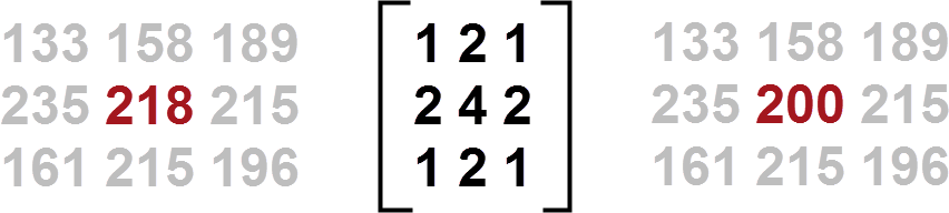
Passing over the data the filter turns the value 218 into 200. Why? Well, if I have my math correct the equation is:
((133 * 1) + (158 * 2) + (189 * 1) + (235 * 2) + (218 * 4) + (215 * 2) + (161 * 1) + (215 * 2) + (196 * 1)) / 16 = 200
i.e. each cell in that 3×3 section is multiplied by its corresponding† kernel value and summed. It’s divided by the sum of the kernel values (16), creating a new value for the centre cell (200).
Basically it’s the average of the surrounding values where each value is weighted by the kernel. So the above kernel gives the centre cell a high weighting (4), adjacent cells a medium weighting (2), and diagonally adjacent cells are given a low weighting (1).
The process repeats, of course, for every cell and every band of every raster feature supplied, producing the desired output. In case you were wondering, the calculation operates only on the original values. When the algorithm processes the next cell (above), its neighboring value is 218, not 200.
† I believe that the “corresponding” matrix value is the opposite one (so for 133 * 1, the “1” is the bottom-right matrix value) but of course here the kernel is symmetrical so it makes no difference.
Filter Types
Different filters have different kernel values and different operation types (some add, some find mean values), and so obviously produce different effects.
Why the above setup produces a blur I don’t know (I swear I used to), but even knowing how it works in general can be important. For example, it shows that the blurring algorithm doesn’t simply reduce resolution (as other methods might) but creates a blur by manipulating the cell colors.
I’ve noticed that kernels like the above, with a positive set of numbers, have a divisor equal to the sum of those numbers. They tend to be blur (smoothing) filters. But I’ve also noticed kernels with negative numbers in them:
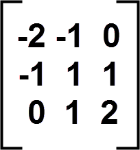
These kernels add up to one and get a divisor of one. These often sharpen the image or detect edges in an image. I believe (I’m no expert) that if the number if greater or less than zero, then the image becomes darker or lighter as FME applies the filter.
Anyway, I think that’s about the limit of my knowledge on filter and kernel theory. Let’s look at how this is implemented in FME…
![]()
Convolution in FME
The FME transformer that carries out convolution is the RasterConvolver. It has the alias of RasterLensProcessor and, for you Quick Add geeks, “nvo” or “rlp” are unique codes to find it!
The RasterConvolver parameters dialog looks like this:
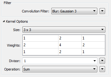
The top drop-down option reveals a whole set of different preset filters:
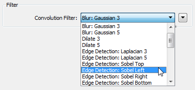
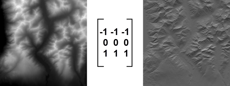
So you can use any of these to process your raster data and create a certain effect. For example, here’s a line detection kernel used on an elevation model:
Picking a fixed filter automatically sets the Kernel, Divisor, and Operation fields. You only change them to create a custom filter. Speaking of which…
Custom Filters
Let’s say I want to produce a custom filter, for example the blur effect is not enough and I wish a bigger blur. Well, that’s easy: I just edit the values in the dialog:
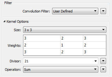
Here I just changed the weights and set the Divisor to match, although I could have set a different kernel size or operation. Incidentally, notice that we allow kernels of 3×3, 5×5, 7×7, 9×9, and 11×11, which are the most common types. We don’t permit non-square kernels.
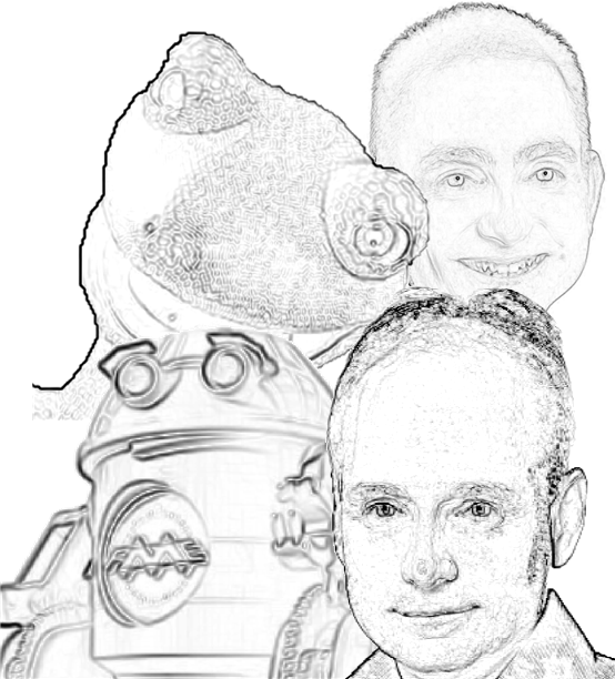
The changes result in (from left to right) Original – Gaussian Blur – User Defined Blur (Click to Enlarge):

Notice that blurring makes the bottom text progressively harder to read. Zoom in and the difference is more obvious:

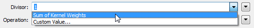
But what do the numbers in the matrix mean, you ask. Well all I really did is shift the weight away from the cell centre to the surrounding cells, by reducing the centre weight and increasing the others. The Divisor is now 21 because the weights add up to 21. To save adding up those numbers, I could also have instead set Divisor to the specific setting of “Sum of Kernel Weights”:
It took me a little research and experimentation to understand the concept and I’m not going to pretend the whole idea of convolution is that simple. However, it is easy enough to experiment with the settings to see what happens, including some of the advanced options…
![]()
Advanced Options
The RasterConvolver has a number of options for advanced control. Their effects will be minor, but possibly important, which is why I mention them here.
Dynamic Kernels
I refer to these as Dynamic Kernels because I can’t think what else to call them. Basically the idea is that you can set the kernel weights through an attribute, a user parameter, or with conditional values. This is done by setting kernel size to “Derived from Weights”:
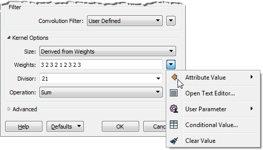
Now I have a text field instead of a grid to define the kernel values, and may use a number of methods. The parameter accepts a list of space-delimited floating point numbers. It’s true that only square kernels are accepted, but you can set of weight of zero to avoid using certain cells and create custom shapes.
Edge Handling
A key consideration is what happens at the edge of images. If each new cell is calculated using its neighbors, then what happens with an edge cell that has no neighbor on one side? Well, FME has a setting for that:
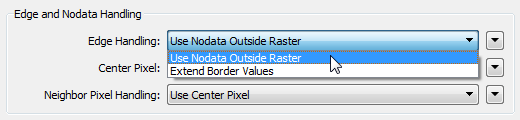
Where a cell is missing FME gives you the option of using either Nodata values, or extending the border values into that empty space. The difference in results (on a 5×5 Gaussian blur) looks like this:
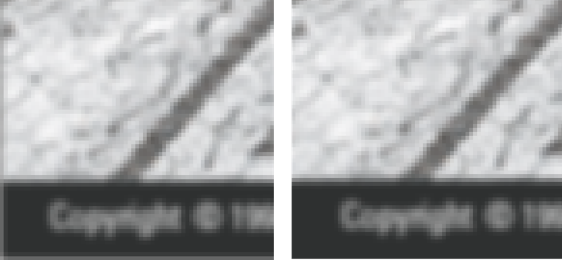
This is the south-west corner, so look at the left and bottom edges. Using Nodata (left image) appears to give a harder boundary, with a clearly defined edge line. Extending the border values gives a softer edge. If I were trying to do edge detection, I think I’d try extending values first, else the raster border might be misinterpreted as an edge (I could well be wrong).
Nodata Handling
And speaking of Nodata, what happens with Nodata values in the raster itself depends on a couple of parameters: Center Pixel and Neighbor Pixel:
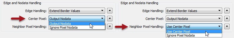
Center Pixel handles the scenario where the pixel being processed is Nodata. It can either be output as Nodata as before, or the Nodata value ignored. Similarly neighboring pixels can be ignored if they are Nodata, or replaced with the Center Pixel value. I suspect you would only ignore Nodata if you knew there were Nodata values; presumably that’s why the defaults are set as they are.
Finally… one advanced option that isn’t controlled by a parameter is the ability to convolve just specific bands in a raster; for example I might want to convolve Red and Green, but not Blue in an RGB image. To do that I just need to precede the RasterConvolver with a RasterSelector, in order to define the bands to be processed.
![]()
Why Convolution?
So having discovered all that, what are the practical uses of this transformer?
Primarily it’s for image processing, such as blurring and sharpening images. You might not think that is so useful, but blurring (smoothing) an image can help hide noise and to bring out details. Let’s take this example where we’re trying to locate ships in the ocean and apply a simple Gaussian blur (click to enlarge):
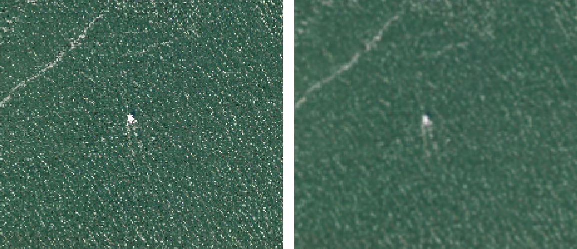
Although the ship we’re looking for is more blurred, the convolution has removed the extreme reflections from the water surface. When I search for highlights to find boats over the whole image (with a RasterExpressionEvaluator) the difference is this (click to enlarge):
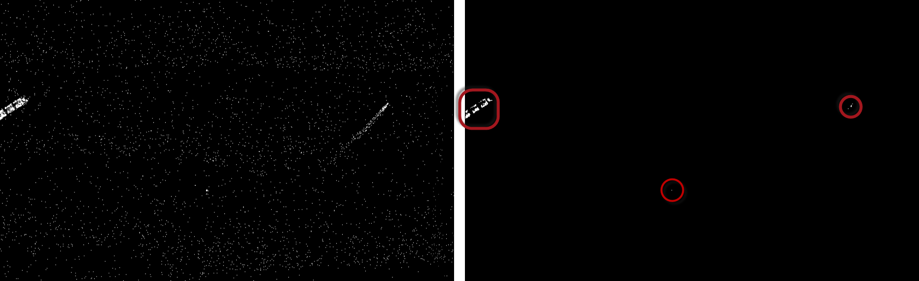
The non-convolved image has thousands of highlights that could be a boat. The convolved image has three clear points. Even the moving boat’s wake got cleaned up.
So kernels like this are useful for image classification. Besides locating ships at sea, they could help you extract built-up areas, assess agriculture inventories, or model flood impacts, for example. Additionally, a series of raster images would show where ships are over time, or even help to track where a particular ship is going or where it came from. Even vehicle detection and tracking might be possible!
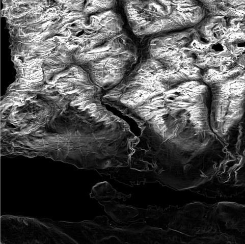
The extraction of vector geometry from a raster image is another common requirement. The first step is usually edge detection, and convolution helps with that too. The RasterConvolver transformer has many different edge detection kernels.
I couldn’t create a spatial example I was really happy with, but I did find that they also can benefit from prior smoothing. And this image is an example of various non-spatial edge detections.
Also, as shown already, the RasterConvolver is not limited to images. It also handles Raster DEMs. For example I found a kernel to generate slopes. I run it on my data and get exactly the same results as the existing RasterSlopeCalculator transformer (in Percent Rise mode). Cast into Int8 for clarity it looks like this:
OK, I say “exactly”. It looks exactly the same in the Data Inspector, but the numbers are slightly different. I figure the two results are just on a different scale. I’m going with the RasterSlopeCalculator as the definitive answer because it tells me what the number means (percentage slope) whereas I’m unsure if the convolved numbers actually represent anything. But still, it shows the sort of thing that you can do with the RasterConvolver on a DEM dataset.
Incidentally my workspace looks like this:
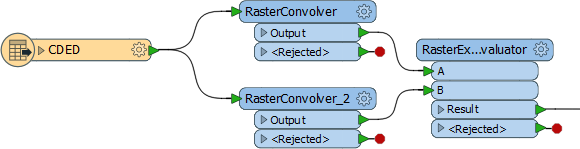
Why the two convolvers you ask? Well, slope/line detection gives different results when applied in a different direction. So I applied it horizontally and vertically in parallel streams, then brought the data back together using the RasterExpressionEvaluator to merge it with:
@sqrt ((A[0] * A[0]) + (B[0] * B[0]))
That’s because I found that expression is better than just averaging the two rasters, as I first tried. You can find this example on our knowledgebase.
![]()
Summary
Merriam-Webster tells me that convolution comes from the same Latin word (volvere, meaning “to roll”) as “convoluted” (meaning complex). I can believe that! This subject is both a little complex and convoluted! But FME makes it easy to pick pre-defined convolution filters and to experiment with custom filters.
I’m also impressed by the speed at which FME processed my data. It took just 22 seconds to read, convolve, and write 40 raster tiles (each 1600 x 1000 pixels in size with 3 bands).
I’ve put two of my examples on our knowledgebase (edge detection and slope calculations) and will put the third on there shortly, in case you want to explore further. Overall there were a lot of user requests for this transformer, so it should be very popular. So go download FME2018.1 and give it a try.
Oh, also notice that the new 2018.1 version of FME also introduces the RasterStatisticsCalculator transformer, for calculating the minimum, maximum, mean, etc values on each raster band or raster palette. I suspect you’ll find that transformer equally useful.

So, yeah, the title and opening are a play on Beatles songs. I wondered if there are any other FME-like Beatles songs and came up with these:
- The Fool on the RasterHillShader
- I Feel Affine(r)
- From me to UUIDGenerator
- Paperback FeatureWriter
- Sgt Pepper’s Lonely Hearts Club RasterBandInterpretationCoercer
- Magical Mystery ContourGenerator

Mark Ireland
Mark, aka iMark, is the FME Evangelist (est. 2004) and has a passion for FME Training. He likes being able to help people understand and use technology in new and interesting ways. One of his other passions is football (aka. Soccer). He likes both technology and soccer so much that he wrote an article about the two together! Who would’ve thought? (Answer: iMark)