 FME 2018 introduced tolerance parameters to a number of transformers. The parameters look straightforward, but there’s a lot more to them than you would think. In actual fact, they amount to a complete change in philosophy in FME’s geometry processing!
You see, one thing we’ve always prided ourselves on is that FME won’t change your data during translation. For sure there are issues to work around. For example, when a format doesn’t support arcs, we write them as lines instead, but the start/end coordinates and the general shape remain the same.
Also, FME is always exact in geometric computations such as line intersections. Very exact. As exact as it’s possible to be in 64-bit computing.
In short, FME never, ever changes the coordinates of your data unless you specifically want that, and always stretches computing to its limits to provide correct transformation results.
Unfortunately – and maybe surprisingly – these techniques do not necessarily provide the best solution in all situations. The nature of 64-bit binary mathematics, combined with a desire for absolute accuracy, can introduce oddities into your data if left unchecked. These usually show up as very very tiny line segments or triangles.
So FME 2018 – through the tolerance parameters – resolves these mathematical oddities. It means breaking some of our cardinal rules, but it turns out that this is a good thing.
This article explains why. It goes into quite a bit of detail. I’ve tried to make it as simple as possible – I wouldn’t understand it otherwise – but if you do find it too technical, skip to the “Practical Use in FME” part near the end.
![]()
Tolerance, Precision, and Binary Maths
Let’s take a look at two issues that occur with mathematics on a computer. First up is the issue of storing decimal values in 64-bit.
Storing Decimals in 64-Bit
Consider the result of dividing ten by three (10/3). How do you represent that result? Well, it’s 3.3333333333 etc. The number 3 recurs to infinity, and you generally round it to whatever precision you want.
Well, some calculations likewise end up recurring in binary. For example, one divided by five (1/5) is 0.2 in decimal; but the result in binary is 0.0111 1111 1001 0011 0011 0011 0011 0011 etc. You can see that the 0011 repeats, and would recur to infinity just as 10/3 does in decimal. The computer rounds it off to the nearest mathematical value which is 0x3FC999999999999A in Hex, or in decimal, it’s 0.200000000000000011102230246252
I can see the effect in FME by placing a 2DGridCreator and setting the column/row width to 0.2:
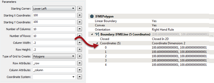
FME scrupulously avoids rounding or changing the numbers it receives, and returns what the computer says is the right coordinates. However, in this case it’s easy to see this is not especially helpful.
So that’s the problem of representing decimal values in 64-bit floating point. The second issue that we face on a computer is that of spatial grid resolution…
Spatial Grids and Precision
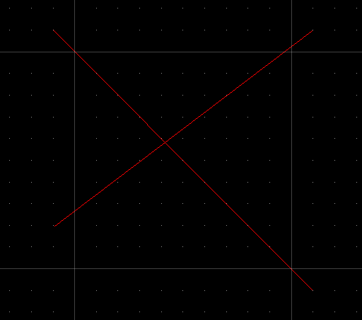
This issue is unrelated to decimal-binary conversions; it’s purely about computing values in binary. FME stores spatial data as 64-bit binary coordinates. If you plot all the possible coordinates as points, you get a grid. If you add lines, their vertices land on that grid:
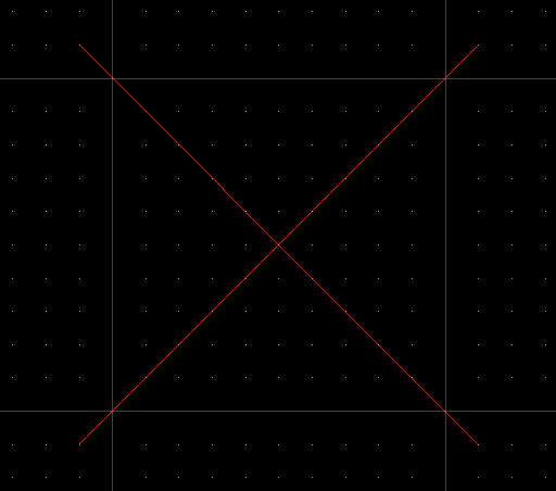
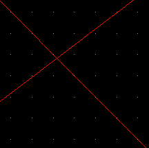
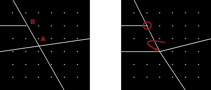
Where do the two red lines intersect? At the coordinate marked on the grid. Easy. However, what happens if the lines intersect like this:
Now where do they intersect? Well if those small dots were 0.1m apart, we could take a guess and say it’s x=0.41m, y=0.59m.
But what if we zoomed until the dots represented 0.01m, and we found that the intersection still didn’t fall on a specific grid point? So we zoom in further and further until each grid interval represents just 0.000000000000001m, and the intersection still doesn’t land on a grid point:
We could do that ad infinitum, but at some point you have to accept rounding off the result. Computationally, FME works in binary and rounds to 64-bits. That’s very precise (for comparison, it’s approximately 17 digits in decimal) and in general that precision is a good thing. That’s because rounding coordinates moves the intersection point slightly. The greater the precision, the less the point is moved by rounding.
But in some cases, there really is a limit to useful precision. When FME returns coordinates with the precision of hydrogen atoms… well we felt that the line had been crossed (no pun intended).
So these two issues are why we implemented some changes in 2018. We’ll take a look at those changes, but first let’s see an example where things would go wrong, and correct a couple of my own misconceptions…
![]()
Tolerance and Ignorance
In the past, if you’d experienced problems with tolerance or precision, I would have suggested one of two solutions. I would have said to either use a CoordinateRounder to round the coordinates or use a Snapper to close off small gaps. It was simple, and it worked. At least, it worked with simple scenarios.
I was very naive though, because I didn’t understand what the problems really were. It’s just a matter of truncating coordinates, right? How hard can it be?! Well, let’s take an example (click to download the workspace) where multiple lines intersect:
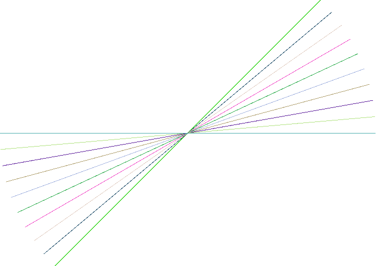
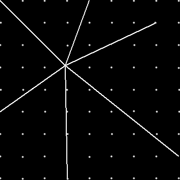
These are just ten lines, each rotated by 10 degrees. Run this through an Intersector without tolerance and what is the result? Ideally it is 20 features, but in fact we get 584! Most of these features are so tiny that even zooming in to the maximum extents of the Data Inspector doesn’t show them.
So what happened? Well, two lines were intersected and their intersection point – not fitting exactly onto the grid resolution – was rounded. Then another line was intersected. It too didn’t quite fit the resolution and was rounded, but it was rounded to a different grid point several nanometres away. This process continues, plus, each time a node is added, the line must be re-checked against the others to see if this no-longer-perfectly-straight line caused another intersection; if so, another newly calculated node is added again!
Finally, at the very heart of the data, after rounding off all our intersections, we get this:
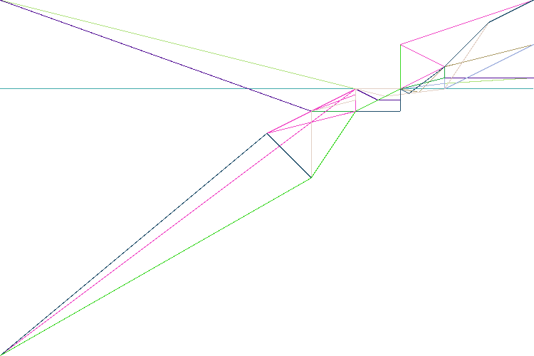
The problem is that by not rounding data to a tolerance, the multiple intersection computations have accumulated errors.
Most of the 584 features are tiny little polygons where intersections intersected. I can even run a LengthCalculator on them to find their size. One of these picked at random is 6.206335383118183×10⁻¹⁷ metres! Since 1×10-12 is a trillionth of a metre, and atoms at their smallest only measure 30 trillionths, you can see the level of precision is a *bit* excessive for your average spatial data!
So that’s what happens when we do nothing to prevent problems in 64-bit computations. Now let’s look at techniques to deal with those problems…
![]()
Tolerance and Enlightenment
During a presentation from our chief scientist, Kevin Wiebe, I found that there are many different solutions, and different products each use different methods. Incidentally, if I mention a drawback with a technique, don’t take it as criticism of these products. Their developers undoubtedly know more about the subject than I do, and will have implemented a technique in a special way to suit their needs. I’m just highlighting the reasoning behind our own decisions.
Anyway, the key to solving many problems in geometric computation is iteration. In fact, iteration, iteration, and yet more iteration!
Snap Rounding
Snap rounding – like the name suggests – is pretty much the method I tried to implement with transformers. You round the data to the nearest grid points, perform processing on it, then snap the results to the grid. It works, but the final snap can result in new intersections to clean up:
Here, for example, the intersection at A snaps to the nearest grid point; however doing so moves the line and creates a new intersection at B.
Fixing new intersections is done by iterating through the process until there are no more intersections: iterated snap rounding this is called.
Overall it’s quick and easy, but there are some drawbacks. Firstly all the data gets adjusted, not just the parts that need to be, and secondly, coordinates can be moved away from their original position. Both of these can (theoretically) lead to problems with broken or collapsed topology; plus the technique doesn’t work very well with arcs.
If you want to know more, there is an academic paper, a simpler description in the CGAL documentation, and actual code on GitHub.
Cracking/Clustering
Cracking/Clustering is a more complex solution. Whereas Snap Rounding works on features individually, cracking/clustering looks at the dataset as a whole to determine how to handle it. Cracking and clustering are carried out using a tolerance value that is usually calculated by the software.
Cracking (if I understand it) carries out intersection and snaps those points onto a grid. Clustering then takes feature vertices and groups them together on one of these intersection points. In this way, you avoid the micro-triangles that plain intersection causes.
Here, for example, are three lines (A,B,C) that need intersection. Let’s try to fix this with snapping:
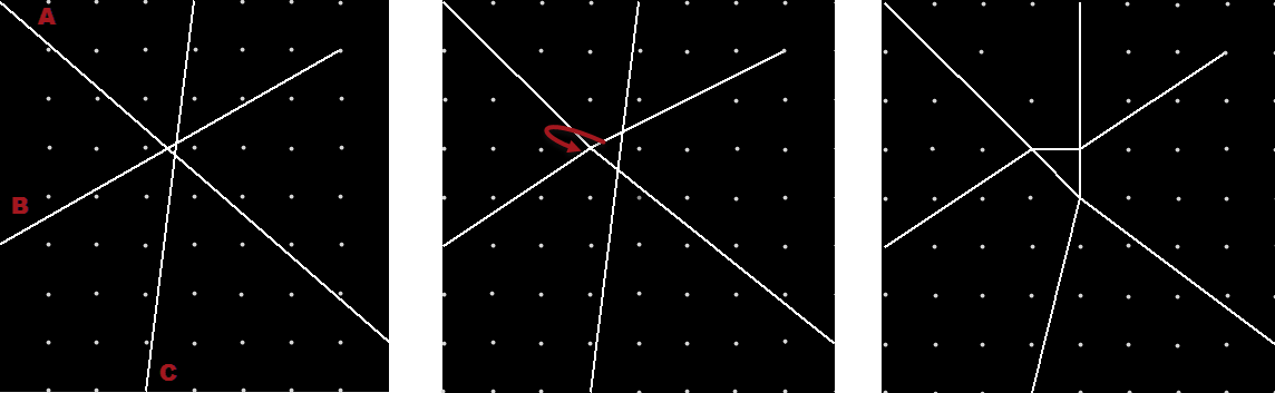
In the first panel are the three lines to intersect. Notice they don’t actually meet at a grid point. In the next panel, A and B are intersected and their intersection point snapped to the grid.
In the final panel, B and C are intersected. That causes line C to move slightly, so that the intersection of A and C is snapped to a new grid point. The result is that the triangular overlap becomes enlarged and actually manifested as vertices. That’s because each intersection is treated separately, and not together. With multiple lines requiring multiple intersections, it’s easy to see how triangles and other strange shapes can be created.
However with cracking/clustering – where the dataset is assessed as a whole – the result would be more like this:
It’s not necessarily the closest grid point to where B/C actually intersects, but it’s a far more sensible solution; and provided the grid interval used is very small, it won’t affect the quality of the output.
Because vertices moved, the process repeats (iterates) until meeting a predefined set of conditions.
If you want to read more about this, Esri has a white paper on the subject.
The FME Approach
At Safe we researched creating our own method, to see if we could improve results. We call our solution Anchored Vertex Adjustment.
The basis of Anchored Vertex Adjustment is to anchor features around points that already existed, not necessarily to grid points. That way features are less affected if nothing has changed, and we move data as little as possible. It also means that features in a network or coverage are more likely to be connected at topologically significant places.
The technique isn’t a two-step process; instead we adjust all the intersections directly as a single step. Using that method, the above example comes out nicely with 20 features all intersecting at the same coordinate:
Let’s see how it’s done by a user in FME…
![]()
Practical Use in FME
First let’s clarify what I mean by precision and tolerance. Precision in coordinates is usually the number of significant digits used to represent a fraction of a unit; for example 12345.6789 quotes a fraction as four (4) digits of precision, and is more precise than 12345.67
Tolerance is more a measure of accuracy. If I have a tolerance of 0.01m, it means each coordinate is only accurate to 1cm. That might be the limit of my survey equipment, for example.
Tolerance often controls or limits precision. That’s because quoting coordinates to 4 decimal places is pointless when I know it’s only accurate to 2 decimal places.
When it comes to FME, the important part is this: FME has (with few exceptions) never applied a tolerance and always given you as much precision as possible.
In some cases lack of tolerance (and maximum precision) is helpful; other cases return better results with a tolerance setting applied to limit precision.
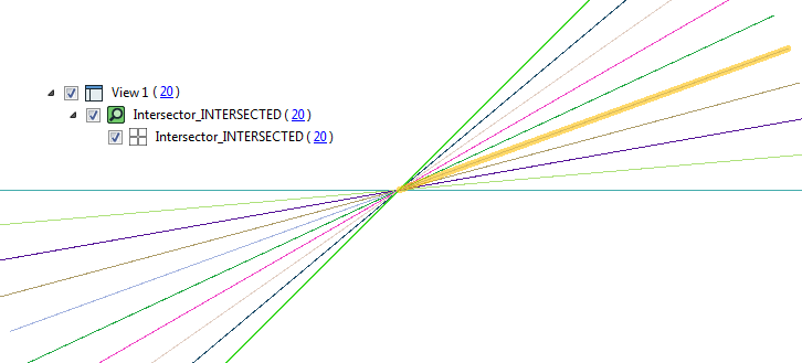
That’s why we created a tolerance parameter in a number of transformers, to give you a choice of which to apply. In the Intersector transformer it looks like this:
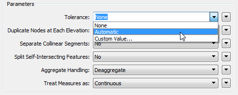
None means that FME works as before. There is no tolerance and FME calculates coordinates to the maximum precision possible. FME does not attempt to resolve the two issues discussed (Storing Decimals in 64-bit, and Spatial Grids and Precision).
Automatic is a mode where FME uses its artificial intelligence to pick a tolerance that applies best to the data.
This setting allows FME to choose more helpful coordinate locations that are within the area of tolerance, preventing issues caused by using excess precision. The tolerance will be very, very small and is not going to adjust your data in any visually significant way. Note that it won’t fix problems with your source data (more on that later).
Example
As an example, let’s take a workspace (click to download) that handles “view cones” in Vancouver. A view cone is an area of land that has a planning restriction so as not to spoil a particular scenic view:
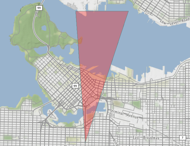
Because Vancouver is such a beautiful city, with a backdrop of mountains to the north, there are LOTS of view cones pointing in that direction:
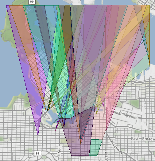
If I want to divide up the land in the city by the number of covering view cones, I would probably use the AreaOnAreaOverlayer:
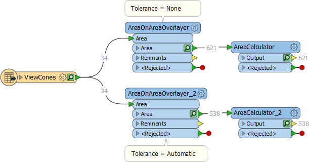
Interestingly, without tolerance I get 621 overlapping areas. Using automatic tolerance I get just 538. Why is that?
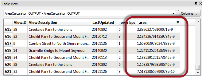
If I run the zero-tolerance results through an AreaCalculator, I can see that the complicated data, along with sticking rigidly to 64-bit mathematics, results in a whole series of polygons that are just an infinitesimal fraction of a square metre:
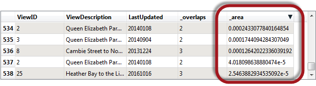
However, with automated tolerance FME works its magic and uses a very small tolerance value in its Anchored Vertex Adjustment method to avoid these ridiculously small artefacts.
How small is the tolerance? Well, I can see that in the log file:
AreaOnAreaOverlayer_2(OverlayFactory): Overlaying with an automatic tolerance of 1.0923954585830338e-8
Now I know what the tolerance is. I also know that computations won’t create any mathematically induced artefacts, or move my data in a way that would break topology.
When to Use Automatic
Generally if Automatic tolerance is available, you should use it. If there is a tolerance parameter available for a transformer, then it is a potentially useful scenario. If there is no tolerance parameter, then it’s not a scenario where tolerance is helpful. So when I notice that the Intersector transformer has a tolerance parameter, but the PointOnAreaOverlayer doesn’t, I understand why. Limiting precision is important in an intersection, but doesn’t matter for a point-in-polygon test.
Additionally, sometimes FME ignores tolerance anyway. A Clipper transformer has a tolerance parameter, but let’s imagine a scenario where all of the Clippees are point features:
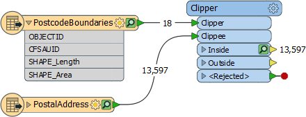
Even if you set Tolerance = Automatic, it’s just a Point-In-Polygon operation, so FME ignores the tolerance.
If, however, the Clippees are area features:
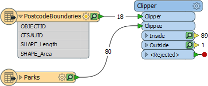
… then tolerance (if set) applies. That’s because it is an intersection operation, and tolerance is useful in that scenario.
In short, Automatic is the way forward, and will become the default option in FME 2019. Only use None when you want data to sustain previous FME behaviour, down to an atomic level of precision!
Custom Value
The option I haven’t yet covered is Custom Value. This means that you can enter your own choice of tolerance.
One use of a custom tolerance is to adjust the automatic parameter that FME generated. For example, even in automatic mode the view cone overlay resulted in some polygons that were very small:
What could I do if I wanted to try and fix those? Well I could take the original tolerance (1.0923954585830338e-8) and increase it a little to see if that helped. I experimented a bit and found that this new tolerance (1.0923954585830338e-5)…
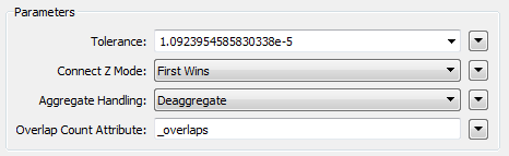
…reduced the polygons further to 533 (instead of 538). Basically it got rid of the five smallest polygons, and I could increase the tolerance further if I wanted.
But another use for manual tolerance is to correct problems with the data itself…
Custom Tolerance for Data Cleaning
As an example, if my view cones didn’t align properly because of bad digitizing, then I could set a tolerance here to force them together. Does that work? Well, yes it does. Anchored Vertex Adjustment repairs errors and maintains topology just as well for large-scale data issues as it does at the micro-level for arithmetic ones.
Let’s take this road network for example:
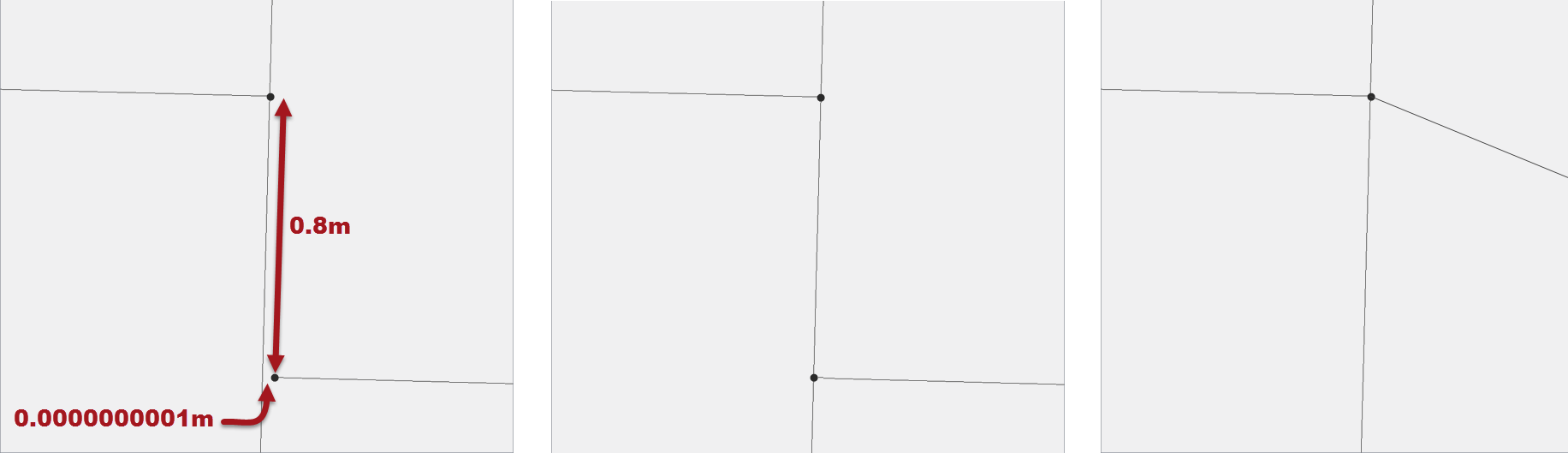
In panel 1 we have the source data intersected without tolerance. Both the very tiny gap and the larger one remain unaligned.
In panel 2 I’ve intersected with automatic tolerance. FME has fixed the very tiny gap, snapping on to a new vertex, so that the line intersects correctly.
In panel 3 I’ve intersected with a manual tolerance of 1 metre, and for a road network that’s a pretty reasonable tolerance. Anchored Vertex Adjustment says that an existing point is better than creating a new vertex (because it doesn’t require a change to the the north-south line) and so snaps to the existing vertex within tolerance.
So, from that we can see that data is cleaned very well at larger scales by setting a manual tolerance parameter. One potential downside is that the road that got moved is now no longer in a direct east-west direction (although I exaggerated the image for effect). So FME has made the least change to the data, at a small aesthetic cost. Such a change is fine at a micro-level because you’d never be able to zoom in small enough to see that; but with a large manual tolerance, it’s something to consider.
In short, custom tolerance is both for adjusting and improving on FME’s automatic tolerance, and fixing gross data errors.
![]()
FAQ
Let me try and anticipate what questions you might have:
- Q) Do all geometry related transformers have this new tolerance parameter?
- A) No. Some may get it in the future but others may never need a tolerance parameter, because their function is not improved by using a tolerance.
- Q) You mention iteration. Should I put my transformer in a loop to iterate the process until it is correct?
- A) No. All of the iteration required is built into the functionality. If you set Tolerance to automatic, then it produces clean data, without you having to repeat anything.
- Q) So is the Automatic functionality complete now? It will always produce the same results?
- A) Yes, it is complete and should be used. However as we learn more, we’ll adjust our algorithm to produce even better results.
- Q) Does coordinate system have any effect on this process?
- A) No. There is no effect from coordinate system. FME carries out computations as if on a plain grid. So if you enter a custom tolerance it’s important to keep the units in mind: a tolerance of 1.xe-5 in metres is obviously greatly different to the same tolerance in decimal degrees.
- Q) Is it really OK for Auto mode to round numbers like this? Won’t it mess up my data?
- A) Yes (it is OK) and no (it won’t mess up your data). Why? Remember there is a difference between accuracy (“My GPS is accurate to 1cm”) and precision (“My coordinates are precise to 7 decimal places”). Auto mode only moves items at a precision well below what your data accuracy could possibly be. Unless your spatial data was literally created using an electron microscope, with picometre accuracy, then nothing we do lessens the worth of your input. Plus we don’t move data at all unless there is a clear benefit; and our Anchored Vertex method means we move it to existing input vertices if one is within tolerance.
Here’s a good joke to expand the last point a little. Imagine a museum tour guide who tells visitors a dinosaur bone is 100,000,003 years and 6 months old. He knows that because he was told it was 100 million years old when he started work there 3 years and 6 months ago! That’s funny. But now imagine a computer that tells you a calculated coordinate is 100.0000035 metres. It’s the same thing. Rounding off either number is not a problem because we know that it’s well within the accuracy of the calculation.
![]()
Summary
 To summarize, FME always returned the results of geometric computation in their purest form, in order to avoid artificially changing coordinates. We returned to our users what their computer’s math chip told us was the correct result.
However, computers are ignorant about what the calculations mean, and it’s up to us to refine their logic to improve our results. That’s what FME’s new automated tolerance option does. It recognizes when it’s better to reinterpret what the computer tells us, within the mathematical error range, in order to avoid oddities in your spatial data.
This new mode aligns FME’s behaviour more closely to other spatial data software, who already use similar techniques by default. But this mode is optional in FME. You can choose whether to apply automated tolerance (like other software), to turn off tolerance in favour of maximum precision (at the cost of possible computational issues), or to enter your own, custom tolerance values.
And that’s why I wrote this post. We wanted our users to know that we’d made a change, but we also wanted to reassure you. FME’s calculations might produce very slightly different results than before, but in a good way. In fact, I’ve been asking for this change for a long time, because pure computation caused me so many problems.
In FME 2018 my geospatial data may no longer be precise to the nearest hydrogen atom, but it’s cleaner, free from mathematical abnormalities, and better suited to any possible use that I can imagine.
There’s a very famous saying that “tolerance is not a sign of weakness, but a sign of strength”. I’d like to think the same applies to FME!

PS: I want to give a shout out to the geometry team at Safe, who created this functionality and then spent hours explaining it to me and providing feedback. They were very tolerant of my inaccuracies (pun definitely intended). You rock!

Mark Ireland
Mark, aka iMark, is the FME Evangelist (est. 2004) and has a passion for FME Training. He likes being able to help people understand and use technology in new and interesting ways. One of his other passions is football (aka. Soccer). He likes both technology and soccer so much that he wrote an article about the two together! Who would’ve thought? (Answer: iMark)